Advances in cryo-electron microscopy (cryo-EM) instrumentation have dramatically increased the pace of data acquisition. Modern microscopes can now deliver multiple datasets suitable for high-resolution structures within a single 24-hour microscope session. However, as data acquisition has accelerated, the bottleneck has shifted downstream, where data processing now increasingly limits throughput.

Public cryo-EM repositories such as EMPIAR provide a unique opportunity to systematically evaluate and refine automated structure-determination workflows. At CryoCloud, we initiated the EMPEROR project to take advantage of this. The EMPEROR project uses the large number of previously deposited datasets to build and stress-test CryoCloud’s end-to-end automation across a wide range of targets, acquisition parameters, and data quality. By reprocessing these datasets at scale, we gain a detailed overview of where automation excels and where targeted improvements are required, allowing us to iteratively refine our workflows toward a more generalised pipeline that is applicable to most cryo-EM targets.

In this blog, we highlight an example from a recent unsupervised workflow benchmark: the gastric proton pump bound to the potassium-competitive acid blocker (P-CAB) revaprazan (EMPIAR-11057).

A clinically relevant membrane protein​

The gastric proton pump (H⁺/K⁺-ATPase) is a membrane protein responsible for acid secretion in the stomach and is a clinically relevant drug target for the treatment of acid-related disorders. Potassium-competitive acid blockers (P-CABs) inhibit the pump by competing with potassium ions at the binding site of the ATPase. P-CABs have attracted interest due to their rapid onset and reversible mode of action when compared with proton pump inhibitors (PPIs).

The dataset discussed here, EMPIAR-11057, captures the proton pump in complex with the P-CAB revaprazan. In the published structure, revaprazan is clearly visible and adopts a conformation in which its tetrahydroisoquinoline moiety inserts deeply into the transport conduit. The biological relevance of this target and the clear ligand density in the published map make it an ideal test-case for assessing the quality of our fully automated processing pipeline.

Fully automated processing with CryoCloud​

We reprocessed EMPIAR-11057 using CryoCloud’s end-to-end automated cryo-EM pipeline, starting from raw movie files and proceeding to a final 3D reconstruction. The workflow ran without manual intervention or iterative parameter tuning. All steps were executed on CryoCloud’s cloud-native infrastructure, which has been purpose-built to optimise job scheduling, stability, and throughput for cryo-EM workloads.

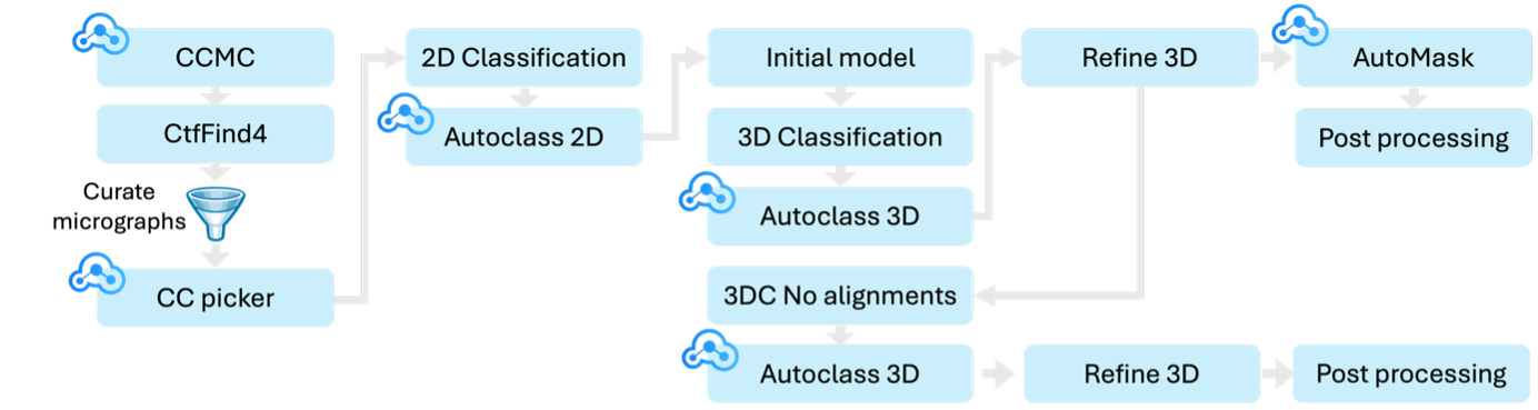
Figure 1. Automated workflow applied to EMPIAR-11057: Steps marked with the CryoCloud logo use CryoCloud's own algorithms: CryoCloud motion correction (CCMC), CryoCloud Picker (CC picker), AutoClass2D, AutoClass3D and AutoMask. Micrographs were curated based on estimated resolution (6 Å cutoff) and ice thickness.

Results: quality and speed​

The automated workflow produced a final reconstruction at 2.6 Å resolution in a total compute time of 43.5 hours, improving slightly on the 2.8 Å resolution reported in the original publication. The final map clearly resolves the bound revaprazan molecule, including density for the tetrahydroisoquinoline moiety within the transport conduit. Notably, the original workflow did not include CTF refinement or polishing, both of which could be added without compromising automation. A subsequent CTF refinement routine on the same particle stack improved the resolution to 2.4 Å.

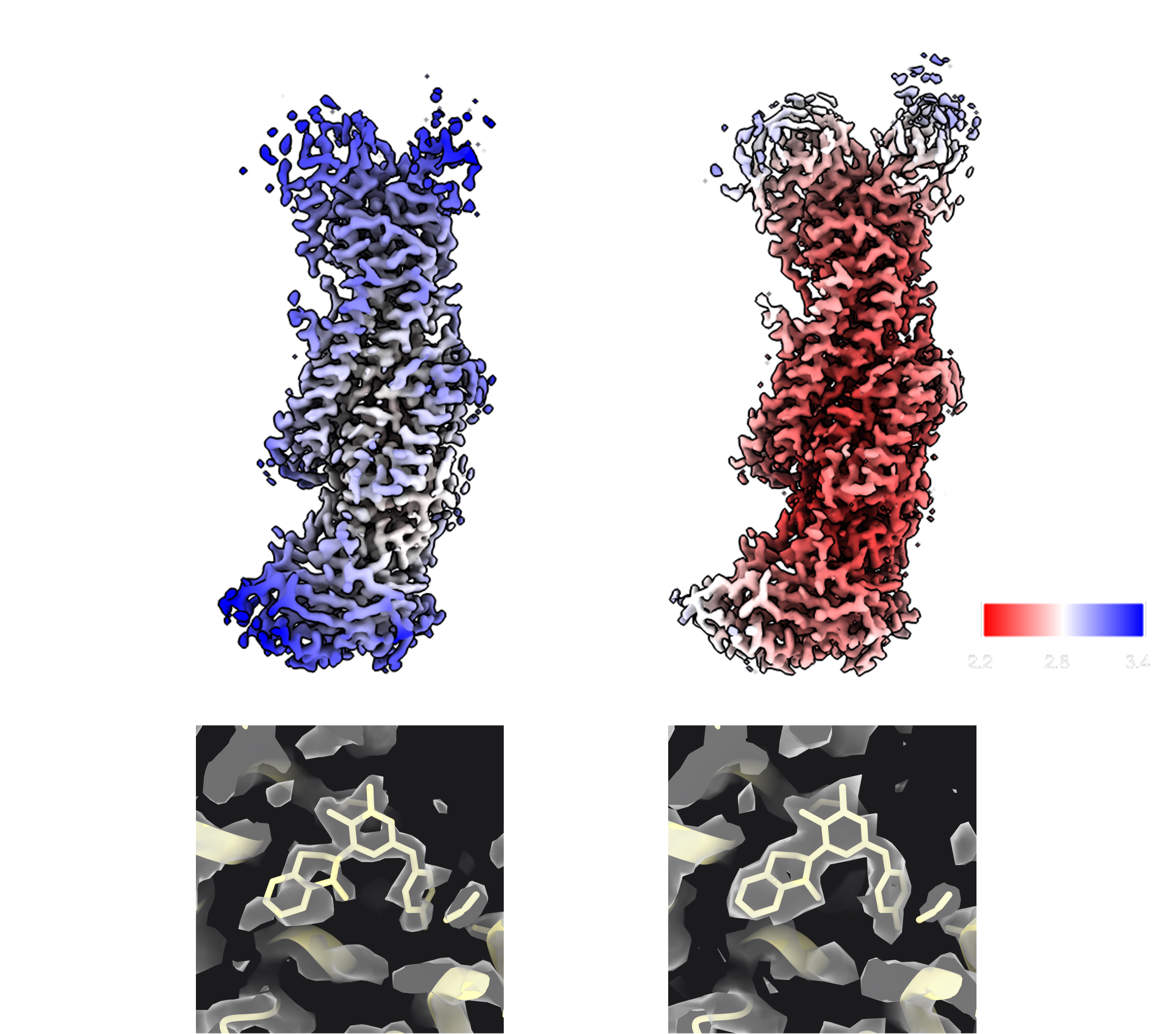
Figure 2. Comparison of outputs from deposited maps and maps generated during automated re-processing. A,B) Map filtered and coloured by local resolution, generated from deposited halfmaps (EMDB-32299) (left) and map filtered and coloured by local resolution generated using halfmaps from final re-processed refinement (right). Colour key for local resolution is shown bottom right. C,D) Density for revaprazan in the sharpened deposited map (left) and the re-processed map (right).

This result demonstrates that automated pipelines can deliver high-quality maps without human supervision and, crucially, on a time-scale that facilitates high-throughput applications e.g. batch processing of screening datasets for identification of optimal sample/grid conditions, or epitope mapping experiments. Importantly, automated pipelines also promote efficient use of computing resources by avoiding manual iterations, reducing the cost per structure in the cloud.

In-house algorithms enable efficient automation:​

Pre-processing​

Our patch-based motion correction algorithm (CryoCloud MotionCorr) processed the raw data at a rate of 3,242 movies per hour, ensuring that motion correction did not become a bottleneck in the automated workflow.

The CryoCloud picker leverages advanced ML models to quickly and accurately pick particle coordinates whilst identifying and masking regions of ice contamination and foil holes in the image.

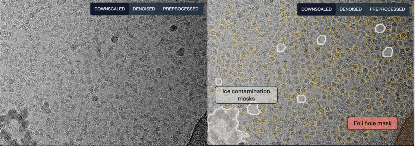
Figure 3. Example output from CryoCloud's ML picker. Unpicked micrograph (left) shown alongside picked and masked micrograph (right). Particle coordinates are indicated by yellow rings. Masks for ice contamination are shown in white, while the foil hole mask is shown in red.

Autoclass2D and AutoClass3D jobs replace the manual selection of classes. Both algorithms use a reference map to identify classes of interest. For 2D, the reference is projected at a range of viewing angles which are then cross correlated with the experimental 2D class averages. The resulting Pearson correlation coefficients are then used as a selection criterion where classes scoring above a pre-defined threshold are taken forward. A similar cross-correlation approach is used in 3D.

Where an autoclass3D job follows a classification job in which no alignment is performed (particle sorting), the selection criterion is no longer based on cross-correlation but rather resolution, with particles belonging to the highest resolution class taken forwards.

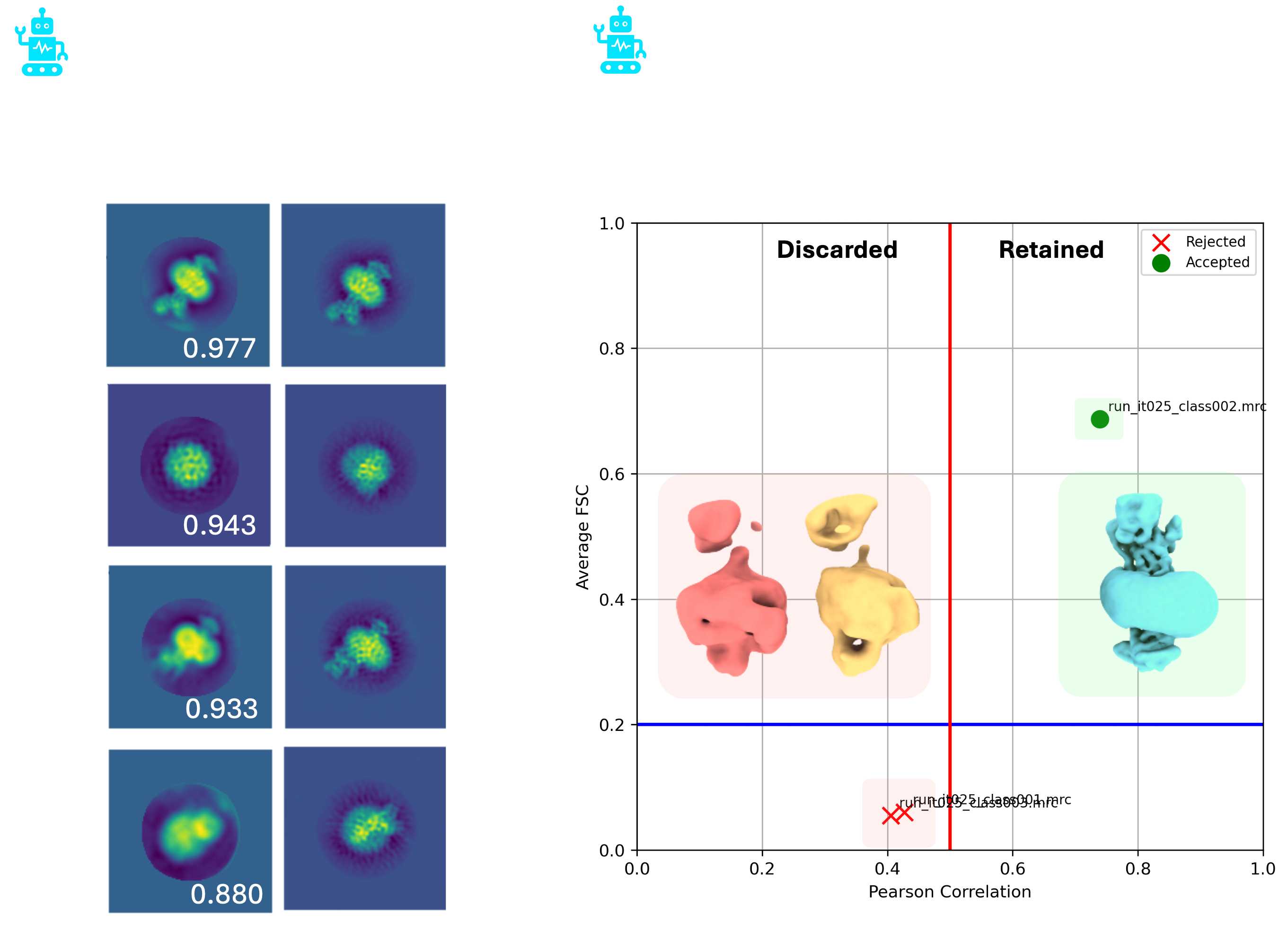
Figure 3. Example outputs from AutoClass2D and AutoClass3D. Representative 2D class averages with their matched reference projections (left). Cross-correlation scores are shown for each pair. 3D class averages that were discared and retained by AutoClass3D overlaid with a plot of their Pearson correlation against average FSC (right). The Pearson correlation threshold for retaining a class is indicated by the vertical red line.

It is important to note that 3D refinement jobs utilise a shape mask (not spherical) by default. The shape masks are automatically generated as part of the workflow by CryoCloud’s AutoMask job. This same tool allows mask generation for use in post-processing operations, removing manual mask creation steps and permitting end-to-end automation.

Automation facilitates throughput and accessibility​

Fully automated cryo-EM processing is not about removing expert oversight, but about eliminating manual steps that limit scalability, consistency, and throughput. By reducing user-dependent decision making while preserving full traceability, automation enables cryo-EM analysis to scale beyond individual datasets and expert users. The reprocessing of EMPIAR-11057 demonstrates the impressive capability of automated workflows, delivering a map of a clinically relevant membrane protein with clear ligand density at a resolution better than originally published, and completed in under two days of compute time without manual intervention.

We're excited to release a new job to the CryoCloud platform: CryoCloud MotionCorr (MotionCorr CC) - Developed in-house and available as part of CryoCloud v2.11 released in early October

Motion Correction: the mother of all jobs​

Motion correction is the first - and often the most computationally demanding - step in the cryo-EM data processing pipeline.

During data acquisition, cryo-EM exposures are not acquired as a single 2D image. Instead, each acquisition consists of multiple raw frames of shorter exposure which are stacked into a movie. Like in photography, the shorter exposures of each frame allow you to account for sample motion without resulting in blurry images. Sample motion arises due to thermal and mechanical stage drift, as well as beam-induced specimen motion. It is these sources of motion that necessitate the alignment of individual frames in the movie before summing up the signal, the so-called motion correction. During this step, patches inside the frame are aligned to each other to estimate the frame shift trajectories, correct for the shifts, and average the signal into one single micrograph with a crisp signal. The accuracy and speed of this step have a direct impact on both data quality and total processing time, which is particularly relevant for large datasets.

During motion correction, the raw data is also significantly reduced in size: movie stacks of 50 or more frames are averaged into a single micrograph, shrinking datasets from several terabytes of raw movies to only a few hundred gigabytes of motion-corrected micrographs. The large size of the raw data is what makes this job computationally demanding - and historically slow.

Up to 4x faster performance using GPU acceleration​

Previously, we have used Relion's CPU-based motion correction job on CryoCloud to align raw movies. While this provided decent speed for smaller datasets and movies with fewer frames and smaller dimension, the motion correction of larger datasets would take several hours.

To speed up this process, we have re-engineered the motion correction job from the ground up. By implementing GPU acceleration, we have achieved a 4x performance boost compared to Relion's CPU-based motion correction.

In benchmark tests using three EMPIAR datasets, MotionCorr CC processed up to 5,000 movies per hour, consistently outperforming Relion's implementation on the CryoCloud platform across all tested detectors, file types and image dimensions.

CryoCloud MotionCorr significantly reduces costs​

Compute costs scale directly with runtime. As such, faster processing also means substantially lower analysis costs. With 2 to 4x speed-up, motion correction jobs on CryoCloud become 50-75% cheaper compared to the legacy Relion implementation which ran on large CPU instances. Or put differently, using Relion's implementation can be up to 3.5x more expensive. This improvement reduced total cloud usage time, making large-scale or high-throughput projects significantly more cost-efficient.

Notably, for small and medium-sized datasets that are used to obtain initial 2D classes for sample screening, the motion correction step can constitute up to 40% of the end-to-end analysis time. By speeding up this step, total readout and processing time are reduced by up to 30%. While these screening datasets are relatively small and their data analysis is relatively fast, the time and cost savings add up over large screening campaigns/multiple projects.

Modern architecture and full downstream compatibility​

MotionCorr CC is fully compatible with downstream polishing and CTF refinement jobs and integrates seamlessly into existing CryoCloud workflows.

It also comes with additional improvements that simplify data handling and improve reliability, such as the detection and exclusion of corrupted image files.

The in-house development of this job also means that we have full understanding and control at the algorithm level, facilitating quality control and the exploration of novel research developments to further improve motion correction.

Key features include:​

• Patch-based, dose-weighted alignment

• Quality-of-life updates like direct target exposure settings for EER files (no more calculator needed!)

• Automatic gain orientation detection (coming soon)

Together, these updates make motion correction faster, more reliable, and easier to run, helping you move from raw movies to refined maps faster.

You can read the full CryoCloud v2.11 release notes here

We are very excited to welcome the second member of the CryoCloud app family: CryoCloud Uploader, or CC Up for short!

CC Up is a stand-alone, OS agnostic tool that runs on your local machine (e.g. microscope support PC), syncs with your datasets in your CryoCloud account, and allows you to create & upload new datasets to CryoCloud. Most importantly, CC’Up supports the live upload of data during your microscope session.

CC Up eliminates bottlenecks from data uploaded post-acquisition​

One major pain-point that we – and many other scientists - frequently experienced during our own research is that data analysis was often delayed by 24- 48h after the microscopy session due to time-intensive data transfers only being started after the completion of data acquisition. Especially in the case of larger datasets (> 10 TB) and limited upload bandwidths, data uploads could take more than a day.

CC Up is able to eliminate this frustrating wait-time in one fell swoop. With CC Up, you can simply specify one or more folders where new files will be written to for live upload. Incoming files will then be automatically uploaded to the specified dataset in the cloud, even while you’re still acquiring data. If you start the live upload at the beginning of a microscope session, and you have a relatively fast upload speed (> 100 MB/s), your data uploads can be finished within 3h of the end of your session – and ready for further processing and analysis on CryoCloud!

CC Up paves the way for live analysis in the cloud​

Another advantage that CC Up provides, is that you can monitor the ingress of new data while data is being acquired at a remote facility. Thereby, you can easily monitor and make sure that everything is going well at the microscope from home or from your office, without needing to request a remote desktop connection. In the near future, the live integration of CC Up with CryoCloud will also pave the way for live analysis in the cloud – allowing you to not only monitor ingress of data but to already get a qualitative readout that can inform your data acquisition!

CC Up runs on all major platforms​

To support uploads independent of the OS and for a variety of use cases, CryoCloud runs on Windows, Linux & Mac. To use it, all you need is a CryoCloud account and a fast internet connection. CC Up is available for all our users no matter the tier. We recommend CryoCloud for both the upload of existing, large datasets from your workstation/ HPC to CryoCloud, as well as for the live upload of data from a microscope support PC.

Are you curious to try CC Up and simplify your data uploads and analysis? Download our state-of-the-art tool below & sign up for a free CryoCloud trial here.

You can find more about how CC Up works in this Guide section.

Download link for CC Up​

Download CC Up for Windows here*

Download CC Up for Mac OS here*

Download CC Up for Linux

*unsigned BETA versions, please follow instructions explained here

This article will walk you through the analysis of a small dataset of a GPCR sample (GLP-1 receptor bound to GLP-1, EMPIAR-10673). The purpose of the analysis is to find suitable parameters, get an idea of your sample quality and obtain a well resolved initial map. All the data presented here was analyzed on CryoCloud, but the principles apply to other analysis pipelines. The article will also give you an impression of CryoCloud’s performance.

Before we dive in, a short disclaimer: for this article we used the dataset EMPIAR-10673 (Danev et al., 2021) containing a highly optimized and well-behaved sample. That means that you might not get comparably high resolutions with your data, but following these steps, you should be able to quickly characterize your sample in regard to particle density, homogeneity, and its propensity to yield well resolved classes. The aim of this article is to highlight important steps during data analysis, and demonstrate that a readout can be obtained quickly without beating your data to death. This will allow you to either get back to the bench quickly to optimize your sample, or, if more data is needed, already plan your next microscope session.

And now let’s get started.

Divide and conquer: select a subset and don’t optimize analysis on a large dataset​

This is one of the well-known, yet often ignored best practices: rather than crunching your whole dataset, you can save a lot of time by choosing a subset that includes an adequate number of particles for initial parameter analysis and screening of your data. I sometimes catch myself or see students ignoring this practice, tempted by the prospect of smoothly progressing through the analysis and quickly obtaining a high-resolution structure. However, the harsh reality is that structure determination is an iterative process, and the majority of datasets will not result in a high-resolution structure right from the start.

For our analysis, we picked a subset of 300 movies from the EMPIAR-10673 dataset, which contains 5,739 movies in total. We selected the first 300 movies from the uploaded dataset (rather than a random subset), to mimic a scenario where one is either waiting for the transfer of the acquired dataset to complete, or analyzing the initial movies that are transferred live from the ongoing microscope session.

We first ran Motion Correction and CTF Refinement, which were both finished in 14 minutes (you can find all runtimes and job parameters at the end of the article), and then excluded micrographs with a maximum resolution lower than 3.5 Å, as done in the publication by Danev et al.. This resulted in 213 movies – a relatively high exclusion rate, but not unusual for the start of a session where acquisition has often not stabilized yet or is interrupted by checks (see Figure S1).

Get your picking right​

Next, we continued with Particle Picking. Unlike in the original publication, where Relion’s 3D reference picking was used, we used Relion’s Laplacian-of-Gaussian (LoG) particle picker. The LoG based picker picked 174k particles in under 2 minutes. We tested reference-based picking in parallel and compared the results later. Reference-based picking took considerably longer (29 min vs 2 min) and visual inspection showed similar results.

Both picking approaches resulted in a comparable number of particles/micrographs and keeper rate after two rounds of 3D classification (260 vs. 306 particles/micrograph and 31.6 % vs. 38.3 % keeper rate for LoG & reference-based picking respectively). The resolution in the final reconstruction, however, was lower for the particles picked using a reference compared to the particle set obtained from the LoG picker (4.17 Å vs 3.54 Å; see Figure S2).

Getting a clean particle set and obtaining an initial low-resolution map​

Next, we extracted the 174,928 picked particles from the LoG picker at a pixel size of 3.03 Å (70 pixel box size). For initial analysis, a pixel size of 2- 4 Å will not only be more than sufficient, but save you time, increase the signal in your data, and help you interpret the results. After extraction, we ran two subsequent rounds of 3D classification with 3 classes each (45 min total). The first round of Class3D resulted in one well-defined class average resolved at 9.24 Å (72.2 % of particles) showing secondary structure features (Figure 1). This class was selected for a second round of 3D Classification, which resulted in a one well-defined class (9.66 Å, 43.5 %) showing a better resolved transmembrane bundle which was selected for subsequent refinement. At this point, we selected 55,366 particles out of the initial set of 174k particle.

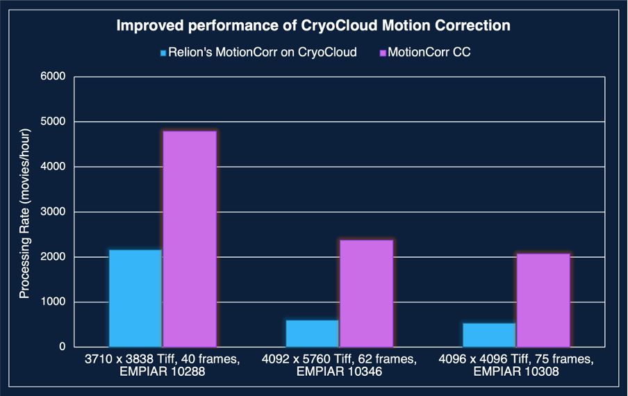
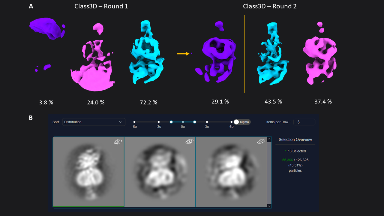
Figure 1: 3D classification of particles and class selection in CryoCloud. A) The set of extracted particles (n= 174,928; box size = 70; pixel size = 3.03 Å) was subjected to two rounds of 3D classification. The well-defined class from the first round was used as input for the second round, resulting in a well-defined class average from a subset of 31% of the total picked particles (selected classes in yellow boxes). B) 3D Class selection panel in CryoCloud - one of several interactive jobs with a custom developed interface, providing sorting of classes and contrast adjustment, and displaying class metadata and total number of picked particles in this case.

Obtaining a high-resolution map​

Next, we extracted the 55,366 particles at a smaller pixel size (1.33 Å, 160 pixel box) and subjected this particle set to two rounds of 3D refinement (41 min total). The first round was run with a mask including the membrane micelle. It resulted in an average resolved at 4.34 Å. For the next refinement round, we created a mask excluding the micelle using the map from the last refine 3D job, and also used solvent-flattened FSC’s during 3D refinement. This resulted in a map at 3.54 Å resolution, which we sharpened using Relion’s Post-Processing. The resulting map shows well-defined sidechain densities as expected at this resolution (Figure 2; you can also download the map at the bottom of the article).

We stopped at this point and did not continue with other post-processing jobs (polishing, CTF refinement). If you did select a subset of your full dataset, achieving this resolution is a good point to apply your protocol to the full dataset rather pushing the resolution of the subset. We will cover that part in our next article.

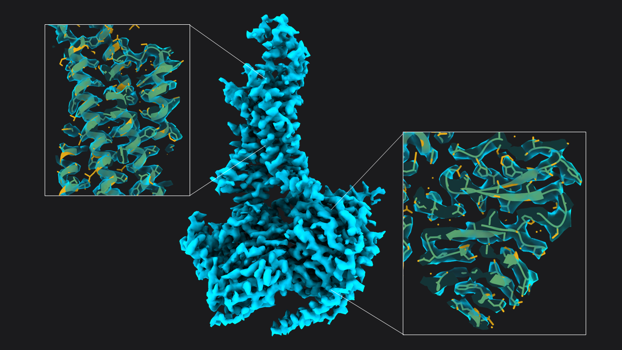
Figure 2: Structure of GLP-1-R bound to GLP-1 at 3.54 Å resolution. Map obtained from ~55,366 particles (pixel size = 1.33 Å, box = 160 pixels) after two rounds of 3D refinement and post-processing. Boxes show slices through the map overlapped with the atomic model (PDB 6x18).

Wrap-up​

Excluding short jobs like selection, mask creation and post-processing the whole analysis (9 jobs) was done in a total runtime of 97 minutes on CryoCloud (Figure 3).

Stay tuned for our next article, in which we will run the analysis on the full dataset, and also include post-processing steps (polishing & CTF refinement) to push the resolution even further. If you have any questions, or would like to leverage CryoCloud for your data analysis, get in touch by shooting us a mail at hi@cryocloud.io.

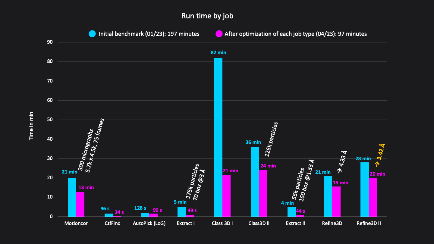
Figure 3: Runtimes of each job in minutes. Excluding short jobs like selection, mask creation and postprocessing the whole analysis workflow consisted of 9 jobs and was done in a total run time of 192 minutes on CryoCloud.

Additional Files​

• Final Map at 3.54A - .mrc file
• Supplemental Data

CryoCloud is live!

And we are looking for a small circle of initial beta testers. If you are interested in using our cloud platform for your #cryoEM data analysis, send us an email at: hi@cryocloud.io